Using Excel’s formula for matrix multiplication (MMULT) is not as straight-forward as using the other built-in formulas provided by Excel. By simply following the MMULT formula wizard, you will get a head-scratching result if you are not aware of the two additional steps necessary in using this formula (or any Excel formula that uses an array as input, such as TRANSPOSE).
Before beginning, we’ll do a quick review of matrices. A matrix is an m x n array of real or complex numbers, where m is the number of rows and n is the number of columns. The matrix is square if m = n and rectangular otherwise. A vector is a matrix of one row or column: a m x 1 matrix is a column vector and a 1 x n matrix is a row vector.1
Two matrices can be multiplied only if the number of columns in the first matrix equals the number of rows in the second matrix. And if so, then the dimensions of the resulting product matrix will be the number of rows of the first matrix times the number of columns of the second matrix.
For example, if Matrix #1 is 2 x 3 and Matrix #2 is 3 x 4, then the matrices can be multiplied, as the number of columns in Matrix #1 (i.e., 3) equals the number of rows in Matrix #2 (i.e., 3). The resulting product matrix will be 2 x 4, which is the number of rows in Matrix #1 (i.e., 2) and the number of columns in Matrix #2 (i.e., 4).
We’re now ready to begin multiplying matrices using Excel. Below are two matrices, a 2 x 3 matrix in cells A1:C2 and a 3 x 4 matrix in cells E1:H3.

As mentioned above, there are two additional steps that need to be done in order for Excel to present the result correctly. First, before using the MMULT formula, you must highlight the area of the product matrix. We now know that the product matrix will be 2 x 4 (per the explanation above). Thus, we must highlight a “target” area of 2 rows by 4 columns. I’ve done that below and accessed the wizard for the MMULT formula.
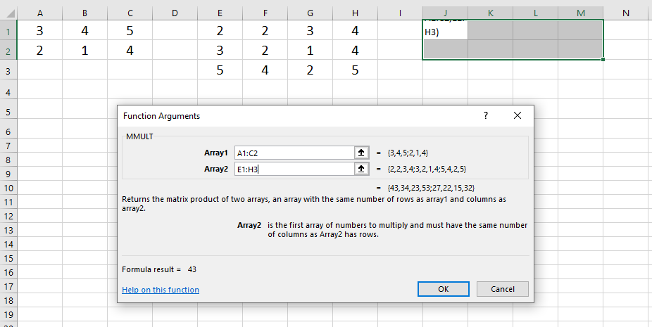
In the image above, the dimensions of the two matrices have been entered into boxes Array1 and Array2 and cells J1:M2 (the 2 x 4 product matrix target area) have been highlighted. By clicking OK, we get the following result:

As can be seen, the full product matrix does not appear. Only a single calculation was done by Excel. In order for the full matrix to be shown, a second additional step must be performed. We must tell Excel that we are entering an “array formula” and therefore, multiple calculations need to be performed. This is done by highlighting the formula in the formula bar and simultaneous pressing CTRL + SHIFT + ENTER.
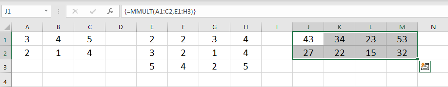
Looking closely at the final image, it can bee seen that the formula in the formula bar is now surrounded by curly braces {}, showing that the formula is an “array formula”. And we now have the full product matrix displayed!
(1) Dennis, Mark R. et al, The Princeton Companion to Applied Mathematics. Princeton University Press, 2015.